
 The tender request for the desalination plant availability analysis (PAA) is becoming a commonplace. Generally PAA shall demonstrate that the offered plant is reliable enough and convince the client that the selected technical solutions are optimized to the availability criteria. Most water companies do not have reliability expert on staff. So the only chance not to be disqualified because of PAA is to outsource it. By the author experience, outsourcing of PAA is not always feasible as the final scholarly report may add some US$ 30,000 to the offer preparation expenses and at least 3-week delay to the offer submission date.
Our experience shows that contrary to the process engineer intuition considering PAA a fancy stuff, at the bidding stage PAA effectively identifies the subsystems with low level of availability and adds substantially to Systems Engineering perspective. Later at the project stage PAA helps compare design alternatives, and track reliability improvement.
The material below explains basic terminology, equations and practical steps of PAA. But first let's have a look at a typical tender paragraph related to availability requirement specification (Australia, 2008). It is called "Redundancy and reliability of desalinated water supply".
As the mine site and associated process plants are solely dependent upon the reliable operation of the desalination plant, and operate on year around basis, a highly reliable supply of the desalinated water is of great importance. Consequently the following requirements apply.
- Plant design and equipment must be of proven performance, reliability and operability.
- In the case of auxiliary systems supplying services to common plant items the failure of a single plant item shall not jeopardize the continued operation of the desalination plant.
- No single component failure will result in interruption of any operation of the plant.
- Sufficient capacity will be available in the system through redundancy, standby capacity or storage, or a combination of these, to allow for diurnal and seasonal variations in demand, system losses, maintenance shutdowns and unplanned outages.
- As a minimum 2 hours of reserve storage capacity for both the mine process water and potable water storage tanks. Others shall provide additional storage for process water at the mine site.
- A plant availability study is to be undertaken by the Contractor to demonstrate a minimum 97% availability will be achieved.
From the excerpt above it follows that the desalination plant shall supply water to the main continuous process. The latter is uninterruptible, so is the water supply even during diurnal and seasonal variations in demand. By the client, the uninterruptible supply may be provided by trade-off between the plant reasonable availability (which shall not be less than 97%) and the water storage capacity. By explicitly defining the storage capacity (2 hours of production rate) the client says that he/she is well aware of the fact that, from the industry experience, for most plant components, MTTR (mean time to repair) is about the same 2 hours.
PAA scope and calculation procedure
Generally PAA is based on a number of assumptions. Some of them are an idealization of the real failure phenomenon (I); others are unearned credit to the client O&M capabilities (O).
- Components are repairable and the failure is always localized and does not propagate outward (I)
- The failure rate is constant (I)
- Preventive maintenance is executed by the book (O)
- The equipment is operated within the range allowed by the manufacturer (O)
- Spare parts stock is maintained well (O)
- The component on-line fault detection covers all the plant systems and critical components.
The bricks of any availability analysis are the component MTBF and MTTR values. Mean time between failures MTBF can be described as the time passed before a component, assembly, or system fails, under the condition of a constant failure rate. Another way of stating MTBF is the expected value of time between two consecutive failures, for repairable systems.
Mean time to repair (MTTR) is defined as the total amount of time spent performing all corrective or preventative maintenance repairs divided by the total number of those repairs. It is the expected span of time from a failure (or shut down) to the repair or maintenance completion.
Maintainability is defined as the probability of performing a successful repair action within a given time. In other words, maintainability measures the ease and speed with which a system can be restored to operational status after a failure occurs.
The availability of a component, system or the entire plant is described by the equation.

As mentioned above MTTR is a sum of unplanned repairs and planned ones. The frequency and duration of the first is probabilistic in nature whereas those of the latter are recorded in O&M books. So it is natural to represent unavailability as a sum of two parts.

The plant availability may be written as follows

 Further we'll focus our attention on unplanned availability, so for the sake of simplicity we'll use 'availability' word without 'unplanned' prefix.
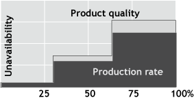
Availability of the desalination plant can be subdivided into the production rate availability and the product quality availability; both are pronounced functions of the plant load. As a rule at decreased loads the plant unavailability goes down, the product quality being less reliable.
Plant: Availability = Availability of Production * Availability of Quality, (5)
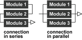
Plant availability is calculated by modeling the system as an interconnection of operating Modules or Blocks in series and parallel, called Reliability Block Diagram (RBD). RBD is an exact replica of the Process Flow Diagram (PFD) used by the process engineer or the Control Flow Diagram (CFD) - starting point for the control engineer. To view PFD, click here.
The following rules are used to decide if modules should be placed in series or parallel.
- If failure of a module leads to the combination becoming inoperable, the two modules are considered to be operating in series. The combined availability of two modules in series is always lower than the availability of either of them.
- If failure of a module leads to the other modules taking over the operations of the failed module, the two modules are considered to be operating in parallel. The combined availability of two modules in parallel is always much higher than the availability of either of them.
The availability of the N modules connected in train is defined as follows.

Where 'a' is the availability of a stand-alone module.
If the desalination plant is resistant to faults and failures of some module, it should be excluded from equation (6). For example, the traveling band screen of the intake stations may be operated for relatively long time with the backwashing system tripped.
Another example is chemical dosing systems; their failure to as low as 50% output for 1 – 4 hours is tolerated well by desalination process. We may say these systems 'fail well'.
The availability of the identical modules connected in parallel depends upon the quantity of operating modules (N) and the one of the standby modules (S).

The same principles apply to the module availability calculation starting from the analysis of the item connections inside the module and collecting data on the item MTBF and MTTR.
As follows from the P&ID excerpt of the intake pumping station, its RBD representation will include 3 identical modules connected in series, each consisting of the pump P, motor M, control valve CV, expansion joint EJ, discharge piping PP and the flow meter FIT.

Table 1 below contains the items typical MTBF and MTTR values found in literature.
Table 1 Typical MTBF and MTTR values for process equipment| No | Component | MTBF, h | MTTR, h | Unavailability*10^6, (1-A) |
|---|---|---|---|---|
| 1 | Pump | 40000 | 4 | 100 |
| 2 | AC Motor | 100000 | 8 | 80 |
| 3 | Control valve | 40000 | 4 | 100 |
| 4 | Expansion joint | 120000 | 2 | 16.6 |
| 5 | Piping | 200000 | 48 | 240 (!) |
| 6 | Flow meter | 270000 | 2 | 7.4 |
| 7 | Module unavailability | 304 (sum of all values) | ||
| 8 | Module in-group unavailability (S=1) | 0.28 (equations 7,8) |
Against sound engineering judgment considering piping a very reliable component not to be included into PAA, table 1 does contain it as well due to very high MTTR. By default all instrumentation of the control loops and the safety interlocks shall be included into module availability calculation.
Actual data may be much worse than those of Table 1 depending on the component design, operational and environmental conditions.
MTBF and Operating Conditions
Motor
The dominating component in the MTBF calculation is the bearings accounting for more than 70% of the motor outages. The standard ANSI-AFBMA Standard 9 – 1990 "Load Rating and Fatigue Life for Ball Bearing" specifies the life of the bearing as a function inversely proportional to the number of revolutions per year and the cube of the load.

Where Ld and La is design and actual loads. For example, MTBF will go up by a factor of 8 if the load is halved.
Second-in-importance factor is the high winding temperature, accounting for about 15% of all the motor failures. If the motor runs too hot, the insulation breaks down much faster. A common guideline states that each 10°C temperature rise above rated temperature cuts insulation life in half. High temperatures also can degrade the grease in the motor's bearings, causing early bearing failure. Bearing or gear lubricant life is reduced by half for every 14°C increase in temperature.
Motor selection for cyclic duty with multiple repetitive starts must take into account the heating caused by starting, load inertia and running load. The heating produced by a large locked-rotor (starting) current might limit the number of starts in a given period of time. During acceleration, a motor draws about 6 times the full-load current, so resistance heating losses (I2R losses) during starting can be 36 times the heating experienced at full load.
Pump
Generally API pumps have twice the MTBF of the none-API pumps. For non-corrosive fluid service about 70% of the pump typical failures are attributed to the failure of mechanical seal, bearing, and coupling. In the pump prediction model, the above-mentioned components are structured serially. Thus, calculated failure rate for pump is a sum of the individual failure rates for these components.
The seal, bearing or the coupling failure rate is mostly associated with the vibration phenomenon. As a rule of thumb these failure rates are inversely proportional to the square of the RMS vibration values. High energy pumps tend to exhibit higher vibration levels and have lower MTBF. Poorly designed piping may trigger hydraulically induced vibrations amplifying the pump's own one.
The seawater pumps working at the temperatures above 25oC (warm service) have the MTBF values lower by approximately 30% (author estimate) due to pitting and crevice corrosion of super-duplex steels.
As follows from table 2 the pump operation far from BEP (best efficiency point) may substantially decrease MTBF.
| No | Operation point deviation, % of BEP | MTBF |
|---|---|---|
| 1 | BEP | 100% |
| 2 | -10%, +5% | 92% |
| 3 | -20%, +10% | 53% |
| 4 | -30%, +15% | 10% |
Variable speed drive
Here dominating factor is the working temperature (defined by the air temperature). Each 10oC rise nearly halves the MTBF value.
Energy recovery devices with cyclic loads (DWEER)
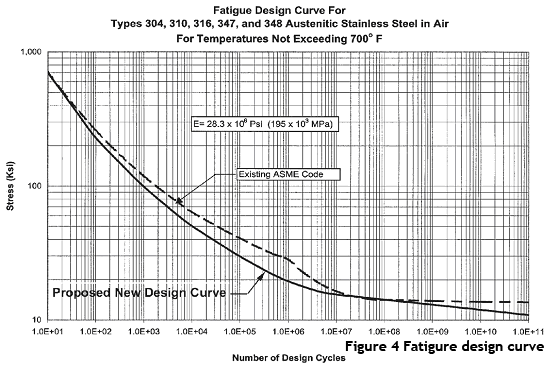
During 25 years of the plant operation DWEER produces approximately 60 million pressure cycles (2 – 75 Barg) acting on the DWEER vessels, valves and the flanges of interconnecting piping. Under the cyclic stress all the materials go through fatigue, its magnitude being illustrated by the ASME curve given in Figure 4 (right).
Independent expert estimates show that due to combined effect of cyclic loads and pitting and crevice corrosion in super-duplex vessels, their expected no-cyclic-load life is decreased from 25 – 30 years to 4 – 10 years.
For check valves installed at the secondary fluid inlet and outlet and working under unusually high load, MTBF value goes down from typical 100,000-200,000 to 25,000 - 35,000 hours.
Gearboxes
Gearboxes are used in travelling bend screens, agitators, skrapers, centrifuges and other rotating equipment. MTBF of gearboxes is a function of the bearing L10 life [Gerhard G. Antony, How to Determine the MTBF of Gearboxes, Power Transmission Engineering April, 2008 ].

RO membranes and pressure vessels
In the past there were attempts to predict the reliability of the RO membrane vessel assembly. Unfortunately this work had been discontinued. The failure data got recently from the desalination plant after 10 years of operation show that broken adaptors and membranes account for nearly 25% of all failures. The RO membrane vessel MTBF value matching the above mentioned failure rate is about 400,000 hours.
High pressure piping
Recommended industrial practices are based on Guidelines for the avoidance of vibration induced fatigue failure in process pipework, 2nd Edition, Energy Institute, London, January 2008 [1].
Likelihood of the high pressure metal piping failure is assessed by the kinetic energy of the fluid flow in piping

In [1] the following classification is the failure likelihood recommended
| Low | Medium | High |
|---|---|---|
 |  |  |
The typical piping design is engineered according to the maximum velocity of 3.5 m/sec corresponding to
![]()
The further step in decreasing the likelihood of the vibration induced failure is the correct selection of the maximum support span. This span is selected according to the recommendations [1] and the LOF criterion (Likelihood Of Failure) of 0.6 (I consider 0.5 too conservative).
Where Dext – external diameter of the piping [mm], T – wall thickness [mm], Lspan – support span [m]. For LOF above 0.6 the piping shall be redesigned.
Example. Find LOF for 8" piping of SCH60 at Dext = 406 mm, T=10.3 mm, Lspan = 4m and the fluid velocity of 3.5 m/sec. From (2) LOF = 0.57 . The LOF for velocity of 3.8 m/sec is 0.67 .
MTTR and Spare Parts Stock
The cited above MTTR values are based on the critical assumption that all necessary spare parts and repair kits are available in stock. So the Spare Parts Stock (SPS) for Corrective Maintenance is a logical extension of PAA: SPS should be sized for each block in RBD. (SPS for Preventive Maintenance is not considered here.)
Just to explain the basic approach in shaping SPS, let's consider a case of 10 identical pumps without standby capacity, having MTBF of 24000 hours (3 years). What shall be SPS for 5 –year operation? As MTBF is the time when roughly 50% of pumps already failed, then the total number of failures is defined by the following procedure.
Failures = 0.5 * 10 pumps * 5 years / 3 years = 8.3 = 9. (12)
Next step is to obtain the pump failure statistics similar to one shown in Table below.
Table 3: Failure breakdown for API OH1 type pumps and AC motors (Ecopetrol S.A.)| Pumps: sample size - 329, year: 2005 | Motors: sample size - 225, year: 2005 | |||
|---|---|---|---|---|
| No | Category | Failure rate,% | Category | Failure rate,% |
| 1 | Seized bearing | 42 | Seized bearing | 76 |
| 2 | Seal leakage | 40 | Winding insulation failure | 12 |
| 3 | Broken shaft | 5 | Circuit breaker failure | 8 |
| 4 | Broken coupling | 4 | Other | 4 |
| 5 | Worn impeller | 3 | ||
| 6 | Worn rings | 1 | ||
| 7 | Other | 5 | ||
So SPS shall contain at least the following
- Seals = 0.4 * 9 = 4
- Bearings = 0.4 * 9 = 4
- Coupling = 0.04 * 9 = 1
- Shaft = 0.05 * 9 = 1
For the pump motors, MTBF is substantially higher (100,000 hours) and SPS leaner. As the motor winding insulation cannot be repaired on site, one motor shall be kept in stock together with four bearings and one circuit beaker.
Module Service Factor
Not all modules are born equal: there exist main and auxiliary modules with batch and continuous operation, overloaded and under-loaded. By analogy with the computer processor, one may say that these modules have different clock speed. To account for the deviation in the component usage conditions, RC introduces the service factor (SF).
For batch auxiliary systems SF is always below 1 and defined as a ratio of the module operation time to the plant operation time. In other words the auxiliary systems are under-clocked. SF may be used to over-clock the modules operating under higher-then–usual vibration rates.
Failure Patterns
As was previously mentioned to simplify PAA, the constant failure rate pattern is assumed. This assumption is not valid for the equipment working under cyclic stress (fatigue phenomenon) and the equipment experiencing severe pitting and crevice corrosion or the pumps under abrasion and erosion frequently observed in the sludge disposal systems.
Crenger automates it all!
The described PAA procedure is fully implemented in GTP; the user does not need to know anything about PAA - it is executed automatically by the button click...
Plant reliability report sample
Internationally Recognized Sources of Reliability Data
| Data Source | Equipment | Available From |
|---|---|---|
| OREDA Handbook | Process Equipment (Offshore) | Det Norske Veritas N-1322 Høvik Norway |
| NPRD-95 – Non Electronic Parts Reliability Data | Mechanical and electromechanical components | Reliability Analysis Center 201 Mill Street Rome, NY 13440 USA |
| PDS Data Handbook | Sensors, detectors, valves & control logic | Sydvest Sluppenvegen 12E N-7037 Trondheim Norway |
| FARADIP III | Electronic, electrical, mechanical, pneumatic equipment | technis@maint2k.com |
| EIREDA Database European Industry Reliability Data Handbook, Electrical Power Plants | Valves, sensors and control logic (nuclear power station data) | EUORSTAT, Paris |